Mixture of Experts Architecture: How Sparse Activation Works

DeepSeek-V3 holds 671 billion parameters. Its technical report states that a single token uses 37 billion of those parameters. That gap of 634 billion parameters is the architecture working as designed.
The design is called mixture of experts, shortened to MoE. It separates how large a model is from how much computation each prediction requires, two quantities that older architectures tied together. That separation is why parameter counts reached hundreds of billions even as serving costs increased only modestly.
This article explains what an MoE layer contains and how sparse activation selects the parts of the network that run. It then covers the published results and what the design demands of the team operating it.
What Is a Mixture of Experts?
A mixture of experts is a neural network layer that holds several parallel subnetworks and routes each input to a small number of them. The subnetworks are the experts. A separate component called the router decides which experts handle which input.
In a transformer, the MoE layer replaces the feedforward block that follows attention. Attention stays dense and processes every token with the same weights.
The choice of location follows from what each component does. Attention mixes information across positions in a sequence, so every token’s representation depends on the others, and that mixing depends on every token sharing one set of weights. The feedforward block processes each position on its own, which makes it the natural place to introduce sparsity.
| Property |
Dense feedforward layer |
MoE layer |
| What the layer holds |
One feedforward network |
Several parallel experts plus a router |
| What processes a token |
The whole layer |
The experts the router selects |
| Parameters used per token |
All of them |
A fraction of them |
| Parameters held in memory |
All of them |
All of them |
| Added machinery |
None required |
Router, plus load balancing during training |
A detailed account of the block this layer replaces appears in this explainer on how transformer models work.
The approach predates the current generation of systems. The 2021 work on Switch Transformers established that sparse expert layers scaled to a trillion parameters, and production systems adopted the design once teams accepted the engineering overhead it requires.
How Sparse Activation Works
Four steps describe what happens to a single token inside the layer.
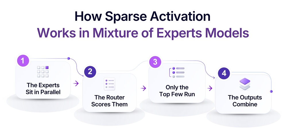
- The experts sit in parallel. Each expert is a feedforward network with the same shape as the others and its own learned weights.
- The router scores them. A small learned layer reads the token’s current representation and produces a score for every expert, indicating how well it suits that input.
- Only the top few run. The layer activates the highest-scoring experts and leaves the rest idle for that token.
- The outputs combine. The selected experts each produce a result, and the layer sums them using the router scores as weights.
The arrangement works because experts specialize. Each expert learns to handle a subset of the inputs the model sees, so the layer stores many distinct patterns and applies a few of them to any given token.
Mixtral 8x7B makes the configuration concrete. Each layer holds eight feedforward experts, and its router "selects two experts to process the current state and combine their outputs." The model holds 47 billion parameters and uses 13 billion for each token.
A common misconception arises, since eight times seven suggests 56 billion. Only the feedforward blocks are replicated across experts. Attention layers and embeddings stay shared, which explains both the 47 billion total and the 13 billion active count.
Expert Granularity Changes the Trade
Mixtral’s eight experts per layer represent one point in the design space. DeepSeek-V3 occupies a different one.
Its report states that "each MoE layer consists of 1 shared expert and 256 routed experts," and that "among the routed experts, 8 experts will be activated for each token." Each expert carries an intermediate hidden dimension of 2048, a size that keeps the individual experts small.
Two choices separate this design from Mixtral. The experts are finer grained, so the router selects 8 of 256 where Mixtral selects 2 of 8, and that wider choice assembles a more specific combination for each token. The shared expert runs for every token and handles computation that all inputs need, which frees the routed experts to specialize.
The arithmetic shows what granularity buys. Mixtral activates 13 of 47 billion parameters, or about 28 percent. DeepSeek-V3 activates 37 of 671 billion, or about 5.5 percent. Finer experts and a shared expert together cut the activation ratio by a factor of five.
A layer with a few large experts therefore behaves closer to a dense one. Hundreds of small experts reduce the active fraction further and pay for it in routing decisions per token.
What the Architecture Buys
The efficiency case rests on one claim. Switch Transformers describes the result as "a sparsely-activated model with outrageous numbers of parameters but a constant computational cost." Parameter count grows while per-token computation stays constant.
That paper measured the gain during training. Models based on T5-Base and T5-Large reached "up to 7x increases in pre-training speed with the same computational resources," and a trillion-parameter model reached a 4x speedup over T5-XXL.
Mixtral shows similar efficiency gains during inference. Its 13 billion active parameters "outperform or match Llama 2 70B and GPT-3.5 across all evaluated benchmarks," with a wider margin reported on mathematics and code generation.
DeepSeek-V3 shows what the approach permits at scale. Its 671 billion parameters trained in 2.788 million H800 graphics processing unit hours, the full training cost its authors report.
What It Costs
Every performance improvement in the previous section is measured in computation per token. The four costs below are measured in memory and in engineering effort, which is why a model that reduces computation can still cost more to operate.
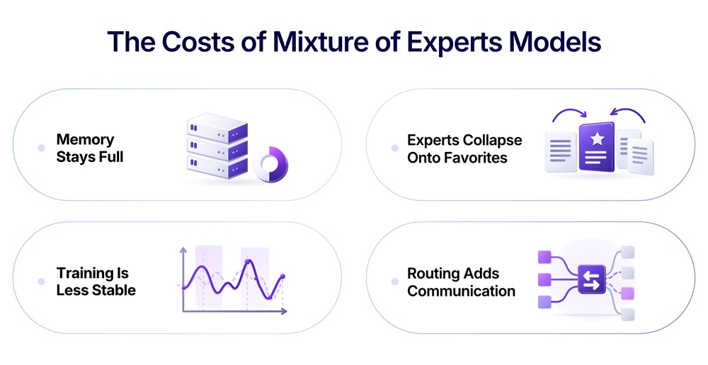
Memory stays full. Sparse activation reduces computation, and every parameter still occupies space on the accelerator. DeepSeek-V3 requires all 671 billion of its parameters resident to compute with 37 billion of them. Compression methods such as those covered in this guide to model quantization address the gap directly.
Experts collapse onto favorites. A router mechanism that concentrates on prediction accuracy alone learns to prefer a handful of experts and starves the remainder. The unused experts waste capacity the model is holding in memory. DeepSeek-V3 "pioneers an auxiliary-loss-free strategy for load balancing," which is purpose-built machinery for keeping the distribution even.
Training is less stable. The Switch Transformers authors report techniques that "help wrangle the instabilities," so plan for a training process harder to manage than a dense equivalent.
Routing adds communication. Experts in a large model are distributed across devices, so tokens travel between them during a forward pass. The same authors simplified their routing algorithm specifically to reduce communication and computational costs. That traffic also ties your serving topology to the model’s expert layout, since the devices holding the experts need fast interconnect.
When a Dense Model Is the Better Choice
Those four costs settle the choice in three situations before accuracy enters the discussion.
Consider model size against your hardware. Where the model you want already fits on your available accelerators, the design adds routing complexity and load balancing work to reduce computation you can afford at full density.
Your serving volume is the next consideration. The compute saving per token holds at any volume, and a server handling a few requests at a time still keeps the full parameter set in memory. Your memory budget covers every parameter while your traffic uses a fraction of the throughput that would justify that footprint.
Infrastructure experience inside your team decides a third case. The instabilities the Switch Transformers authors describe require engineers who can diagnose them during a training run, and a dense model of equivalent capability trains along a better understood path.
Below the scale where your target parameter count exceeds the computation you can afford on every token, a dense model reaches the same result with less machinery to operate.
What This Means When You Deploy One
Two numbers drive your decisions about an MoE model, and they answer different questions.
The total governs your hardware. All parameters must be resident for the router to reach any of them, so your memory budget follows that figure with no discount for sparsity.
The active count governs your throughput. Latency and cost per token track the parameters that compute, so your throughput estimate follows the active count alone.
Reading only one of the two produces errors in opposite directions. A team that sizes hardware from the active count exhausts memory before serving a request. Estimating cost from the total creates the reverse problem, where a workable model appears unaffordable and the team declines it.
Batch composition adds a third consideration. A single token activates two experts, and the tokens inside a production batch route independently, so a full batch can touch every expert in the layer. Your per-token activation figure describes one token and understates what a busy server holds active at any moment. Load testing at production batch sizes shows you the difference.
Monitor expert utilization after launch. A router that concentrates on a subset of experts in production produces degraded output on the inputs the starved experts had specialized in. Log the distribution of expert selections across a sample of live traffic to confirm that the balance achieved during training still holds.
A second lever on inference cost is the computation you spend per request, which this guide to
test-time compute examines.
Conclusion
Mixture of experts breaks the link between a model’s size and the cost of using it. Hundreds of billions of parameters became affordable to serve once that link was broken.
The design asks for a full memory footprint and a harder training process in return, along with load balancing machinery specific to sparse layers.
Every technical report of this kind publishes the total and the active figure together, and the two answer different questions. Size your hardware from the total and estimate your throughput from the active count.